Assessing Land Use
Collect Earth provides an easy system for using freely available satellite imagery in Google Earth, Bing Maps, Yandex and others as well as Planet and Google Earth Engine to classify land use and assess land use change over time.
Land use classification schemes can vary greatly by country or program. Several country-specific versions of Collect Earth software have been configured, as well as versions consistent with leading international guidelines (e.g. IPCC, Food and Agriculture Organization Forest Resources Assessment, etc.).
Land use classification schemes can vary greatly by country or program. Several country-specific versions of Collect Earth software have been configured, as well as versions consistent with leading international guidelines (e.g. IPCC, Food and Agriculture Organization Forest Resources Assessment, etc.). This tutorial explores the basic functionality of the software and its supporting tools.
Click on the steps below to view more details.
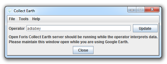
Launch Collect Earth. In the main Collect Earth window, type in your operator name (between 6 and 50 characters long). Then click Update.
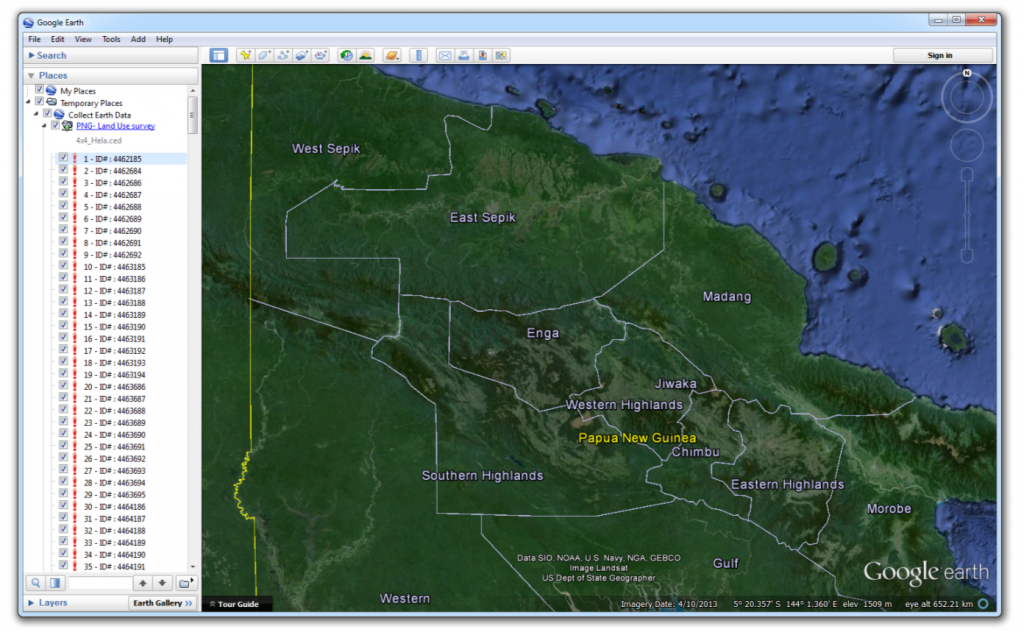
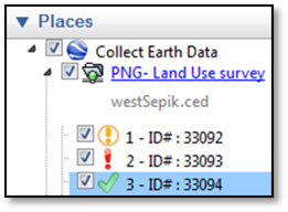
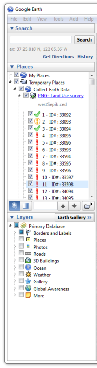
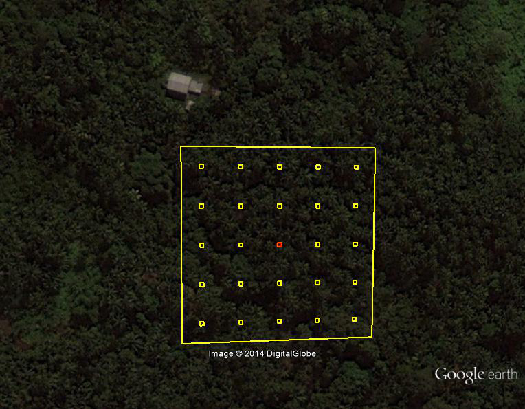
Collect Earth will automatically launch Google Earth. Collect Earth organizes sampling plots for Papua New Guinea in sub-national units. In the Places panel on the left, the Collect Earth Data folder contains PNG Land Use survey sampling points from Hela Province arranged along a 4° x 4° grid. Data for each of the country’s 20 provinces are saved in separate Collect Earth Data (CED) files.
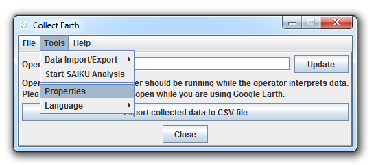
To enter data for a different province, return to the main Collect Earth window and select Properties under the Tools tab.
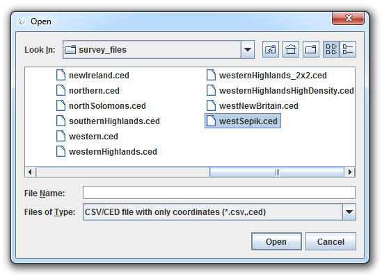
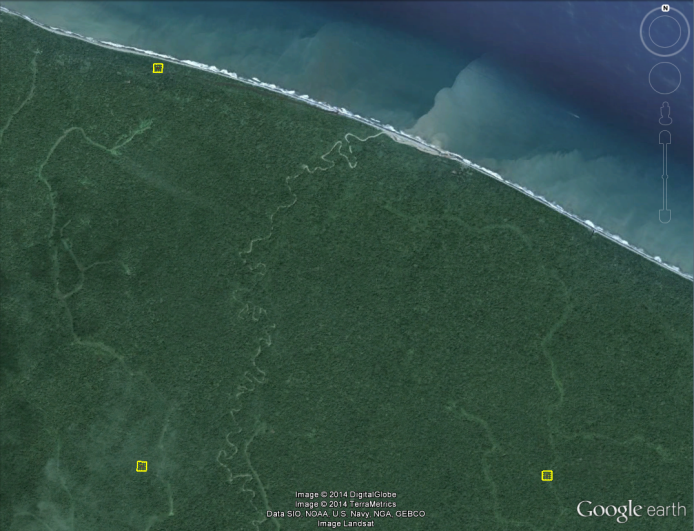
Under the Sample data tab, click Browse to view the CED files available for other PNG provinces. Scroll to the end of the survey files list, select West Sepik and open the file.
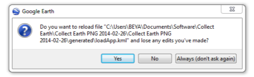
To enable Google Earth to reflect the changes you have made within Collect Earth, click Yes to reload the data within Google Earth and click OK to confirm the changes.
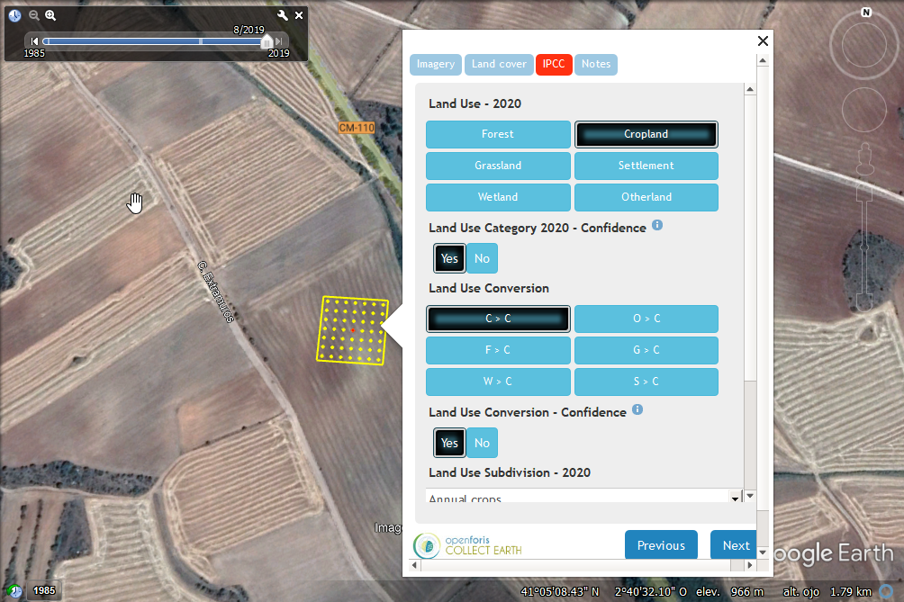
Use the Collect Earth dialogue box to enter land use information for the plot.
Land use classification schemes vary by country. To facilitate national reporting to the UNFCCC, the country-specific versions of Collect Earth present land use classes through a land representation framework recommended by the IPCC. The data entry prompts within Collect Earth will vary accordingly. This framework outlines six main land use categories that more detailed land use sub-divisions will fall within.
Land use sub-categories indicate the conversions from one land use to another. The year of the change is significant for interpreting land use change dynamics and estimating emissions from land use change.
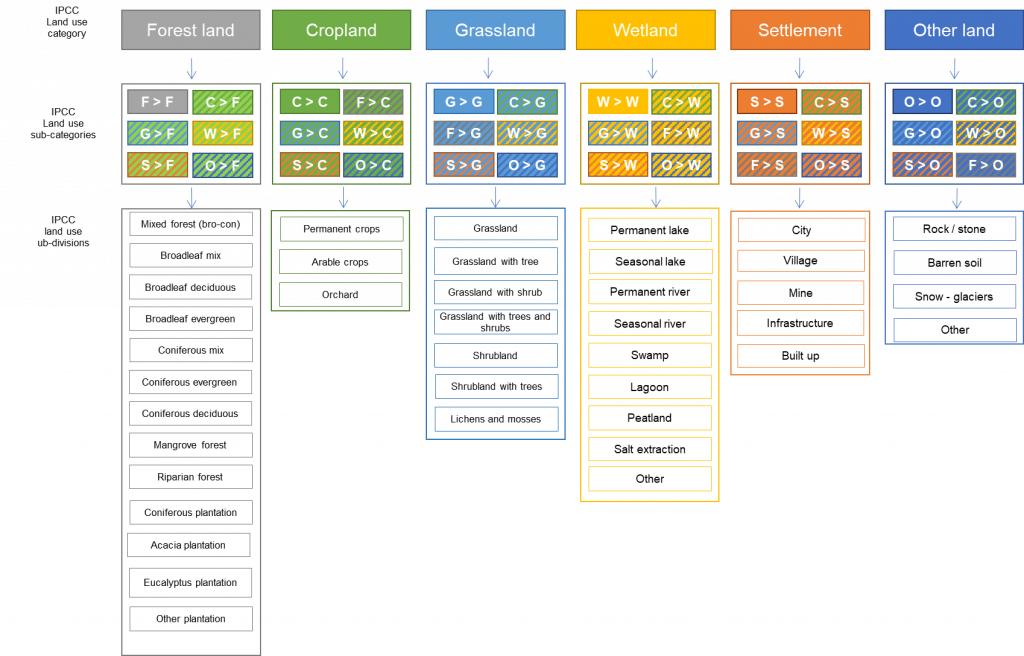
The Accuracy options allow users to indicate their level of certainty with their selections. Accuracy is a required field in the land use category, land use sub-category and land use sub-divisions sections. The Land use sub-divisions are detailed land use classes that more closely represent realities within a country or an area of interest.
The Canopy options include quantitative and qualitative descriptions of forest canopy cover. The cover percentage can be calculated from the ratio of plot points under canopy cover to the total number of plot sampling points (25). Uncertainty may arise where no high spatial resolution imagery is available for the plot area. If uncertain, select No under the accuracy option. The Site description contains information related to accessibility and elements located within the sampling plot.
If Human impact in the plot is apparent, indicate the type, accuracy, grade (or level) and the first year the human impact became apparent within the historical satellite imagery of plot.
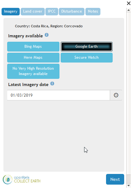
Under RS Data, select the type of satellite imagery that was used to assign the sampling plot to one of the six basic land use categories. The imagery used should be the most recent imagery available that is of sufficient spatial resolution to assess land use.
Click Submit and Validate to save the data you have entered.
In the Google Earth Places panel, a red exclamation mark appears beside plots without data. The exclamation mark turns yellow when data is entered but not saved. A green check appears once the data has been submitted and validated.
Use “Validation Rules” within Survey Questions to Limit Human Error
“Validation rules” can be coded into the survey to establish parameters that need to be met for a certain response to be valid, helping to reduce the potential for human error. For example, the tree cover percentage for a sample plot can only be a numeric response between 0 and 100; if a data collector’s response is non-numeric or exceeds 100, an error message will result. At a minimum, we recommend that you establish rules that ensure that all key questions in the survey are answered. A common source of error occurs when data collectors accidentally skip a question when moving quickly through a survey. To prevent this error from occurring, a rule can be set up such that the data collector cannot save their responses and move on to the next sample plot until the missing response has been provided.
The plot layout, size and spatial distribution can also be modified to maximize compatibility with a country’s existing or planned forest inventories.
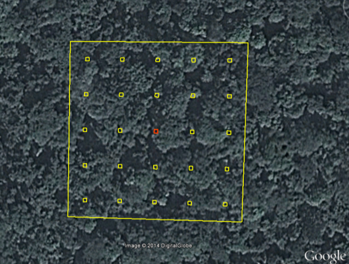
In the PNG version of Collect Earth, plots are arranged along a 0.04° (4.45 kilometer) grid.
Each plot is 100meters long and 100 meters wide, with an area of one hectare (10,000 square meters). Each plot contains 25 sample points along a 20 meter grid
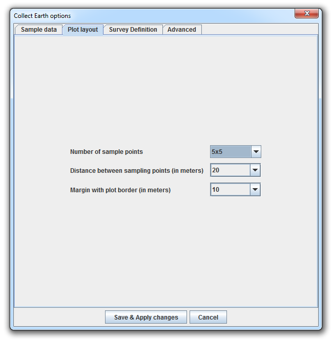
In the main Collect Earth window, under the Plot layout tab, the number of sample points within a plot can be adjusted, along with the distance between sample points and the size of the margin between sample points and the edge of the plot. To change the distance between plots (and create a new grid), see the tutorial on Sampling Design with Saiku Server.
Collect Earth data files can be exported as CSV and XML files. For the first option, click on Data Import/Export in the Tools menu, and select Export data to CSV. Name and save the file.
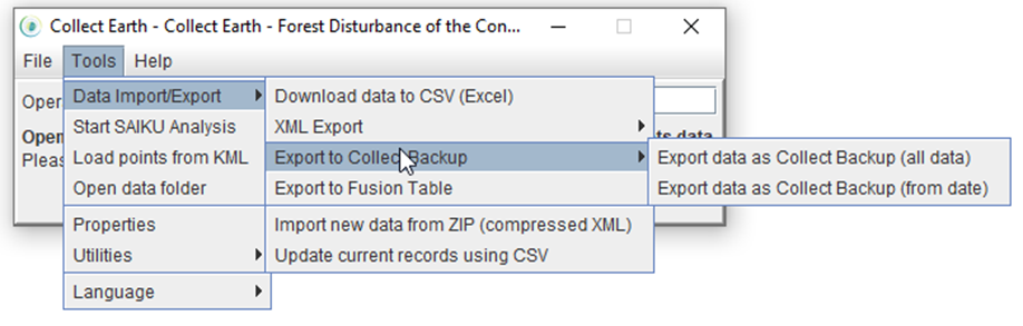
The CSV file, which can be opened in Excel, tabulates all of the data that has been entered in Collect Earth, including data that has not been actively saved and validated. The plot coordinates and the operator name are also saved. The user may save all the collected plots from a given date.
XML is the only format that is configured to save all of the Collect Earth metadata in addition to the data manually entered by users. Click on Data Import/Export in the Tools menu, and select Export data to XML (Zipped). Name and save the file.
The command for importing data from XML is located in the same Tools menu.
Useful settings and features in Google Earth
Google Earth serves as the main interface for Collect Earth software. Adjusting certain settings and familiarizing yourself with the basic functionality of Google Earth can enhance the experience of using Collect Earth. A few tips are below.
Click on each heading to view more details.
After launching Collect Earth, data from the application will appear within Google Earth’s Places Panel on the left-hand side. The Search Panel above and the Layers Panel below will rarely be used. Minimize these panels to display more Collect Earth data.
Click on the Search bar and the Layers bar to minimize these panels. The new view maximizes the length of the Places Panel, which contains the Collect Earth data.
Use the Find tool at the bottom of the Place Panel to search for a particular plot. Always use the unique plot ID rather than the plot number, which will vary by region. Type the plot ID#. If the ID# is present within the dataset, Google Earth will scroll to and highlight the plot.
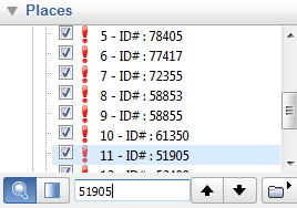
If the ID# is not present, the search field will be highlighted in red.

Google Earth navigation settings control the Fly-to-speed and the way you way you approach each site. The Fly-to-speed is particularly important when working with slow internet connections. A fast fly-to-speed can reduce the amount of time one waits for the imagery of the sight to load.
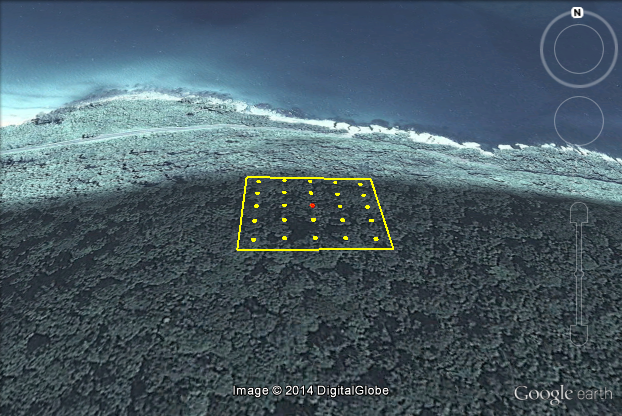
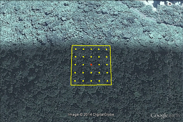
Google Earth’s default navigations setting may tilt when arriving at a site. The titled view on the left makes it difficult to clearly view all sampling points within a plot and assess land use.
| 30 View with tilt | View without tilt |
 |  |
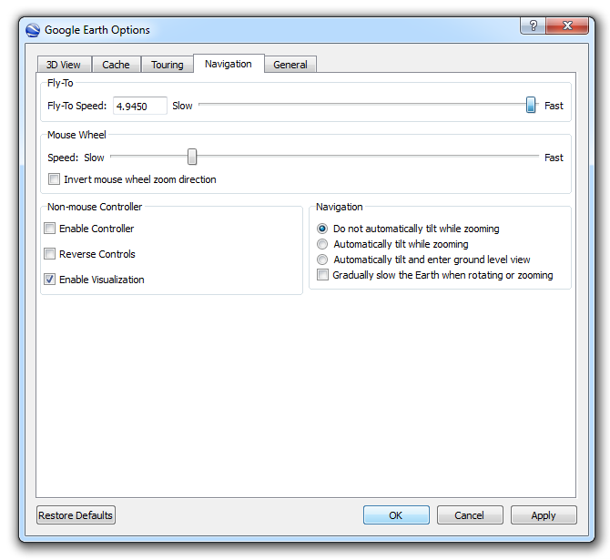
Adjust the navigation settings by clicking on Tools in the Google Earth toolbar and then Options.
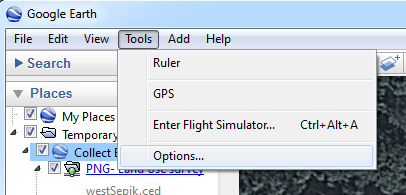
- Drag the Fly-to-speed slider from Slow to Fast.
- Select Do not automatically tilt while zooming.
- Click OK to save the changes.
Measuring distance within Google Earth can be useful for determining the plot accessibility. To measure distance, click on the ruler in the Google Earth taskbar.
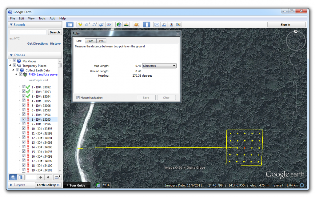
A target box will appear instead of the normal pointer arrow. Click once on the point in the center of the plot. Then click once on the center of the road to draw a line for measurement. The length of the line will automatically display within the Ruler box.
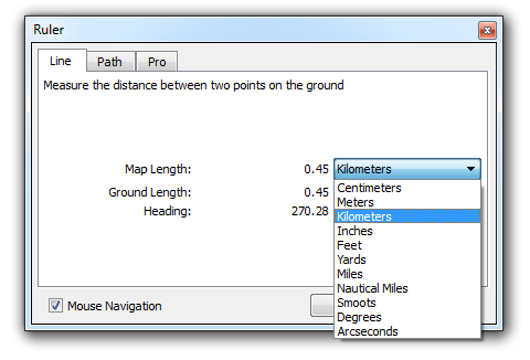
The unit of measurement can be changed by clicking on the dropdown tab beside Map Length. Select kilometers.
In the Collect Earth dialogue box, select the approximate distance and the bearing from the plot toward the access point. You can also type additional details that may be helpful when planning the ground-based forest inventory.
At the bottom of the Google Earth navigation window, the date of the imagery appears beneath the imagery copyright year and source. Google Earth default settings present the date in MM/DD/YYYY format, but the data format may vary with the language setting. For example Spanish and French Google Earth display data in DD/MM/YYYY format.
Imagery date: October 30, 2010
Imagery source: Digital Globe
Details for the most recent image used to classify land should be entered in the Collect Earth dialogue box.
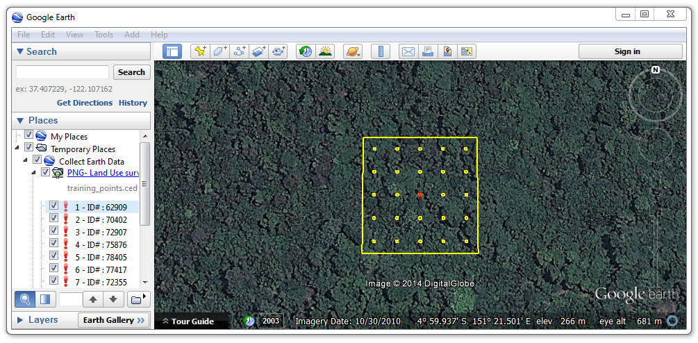
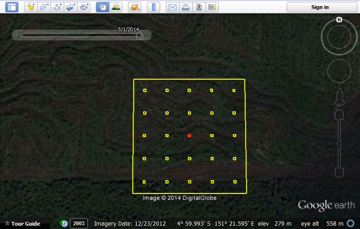
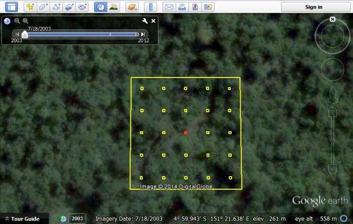
Click on the clock in the Google Earth toolbar to browse historical imagery. Occasionally, more recent imagery may also be viewed with this tool. For plot ID# 62909, imagery is available from 2014 and 2003.
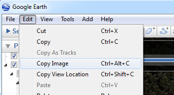
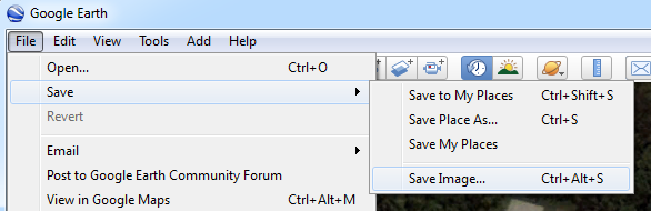
When working with a team to conduct a land use classification, it is important to have a common understanding of how various land uses will appear in satellite imagery. Google Earth imagery can be exported in jpeg format, which may be an easier and lighter (in terms of file size) way to share views of various land use classes.
There are two ways to export images as jpegs:
Under the Edit menu, select Copy image. The jpeg image can then be pasted in a different program.
Alternatively, you can save the image using the File menu.
The jpeg will contain the view from the navigation frame without the navigation tools and taskbar. The image below is an example of a coconut plantation near a dispersed settlement in Papua New Guinea. This land use class may be more easily recognized if Collect Earth operators can view sample imagery before classifying plots.
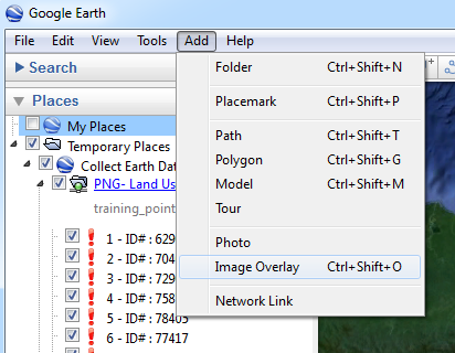
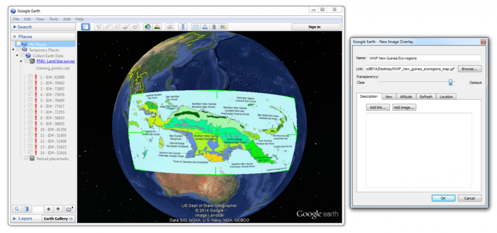
Existing maps that may facilitate land use classification can be added in Google Earth as overlays. The instructions below apply to maps and images without a spatial reference system. For georeferenced rasters, see section 5.3 for guidance.
Click Add in the Google Earth taskbar and select Image Overlay.
Type in a name for the image you will add. Then browse for and open the file. WWF New Guinea Ecoregions has been added below.
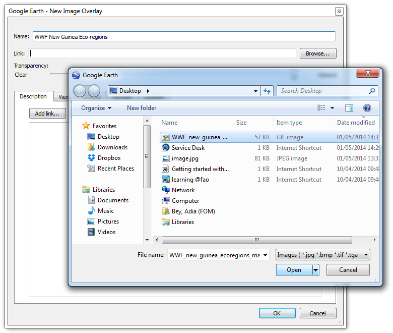
Before adding the image, notice the green lines that will be used to control the image.
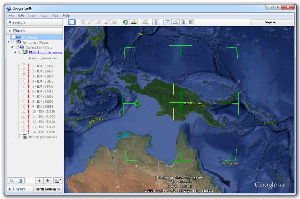
Once the image has been added, use the image controls and the layer transparency slider to adjust the size and positioning of the image.
- Pivoting the diamond around the cross rotates the image
- Select Do not automatically tilt while zooming.
- Dragging the corners inward and outward adjusts the size and stretch of the image
- Dragging the center cross moves the entire image
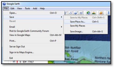
Image overlays and other supplementary data should be saved as KMZ files. (Collect Earth data is handled differently. It is automatically saved to a database and it can manually be exported as a CSV file, Fusion Table or XML).
To save a single layer, right click on the layer and select Save Places As. Add a file name in the dialogue box that pops up and click Save.
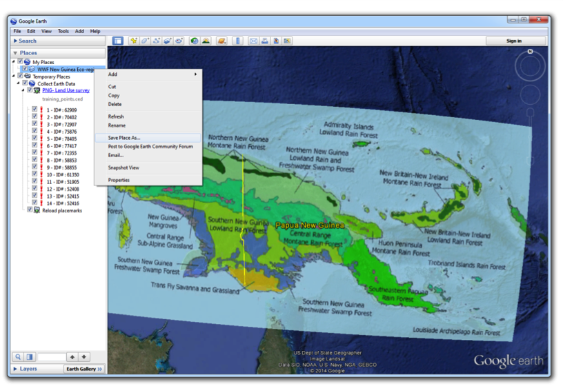
Alternatively, you can select Save multiple layers by selecting Save places as under the File menu, or by right-clicking on a entire folder (that contains layers) within the Places panel.
New perspectives with Bing Maps
Bing Maps is a web mapping service provided by Microsoft. Through Bing Map, high spatial resolution satellite imagery from Digital Globe can be viewed and used for land use assessments. Collect Earth plot locations have been linked with Bing Maps because the latter web mapping service has a slightly different geographic coverage. Some plots, such as plot ID#52416, have high resolution imagery in Bing Maps where only Landsat imagery is available in Google Earth. To zoom to the plot location in Bing Map, click anywhere within the plot in Google Earth.
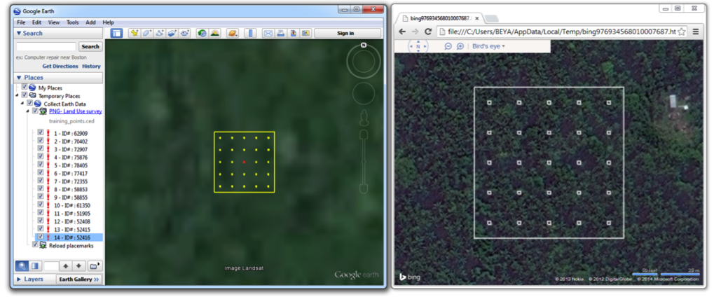
In the image above, Google Earth features medium spatial resolution Landsat imagery of plot ID#52416, while Bing maps provides high resolution Digital Global imagery over the same area. The Digital Globe imagery makes it easier to identify the vegetation as coconut trees (agricultural land) rather than forest land.
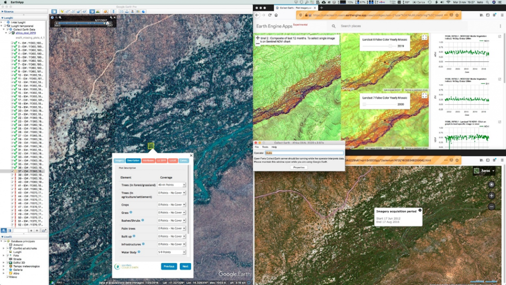
Google Earth Engine is a web platform for processing satellite imagery and other Earth observation data. Google Earth Engine provides free access to coarse, medium and high spatial resolution satellite imagery acquired over the past forty years. Various types of pre-processed imagery can also be used for land use analysis.
One of the most useful land datasets available through Google Earth Engine is the Landsat Greenest-Pixel top of atmosphere (TOA) reflectance composite. These composites, which are available for Landsat 4, 5, 7 and 8, are created by drawing upon all images of a site for a full calendar year. The greenest pixels, with the highest NDVI (normalized difference vegetation index) value, are compiled to create a new image. These composites are particularly useful in tropical forest areas that may be prone to frequent cloud cover.
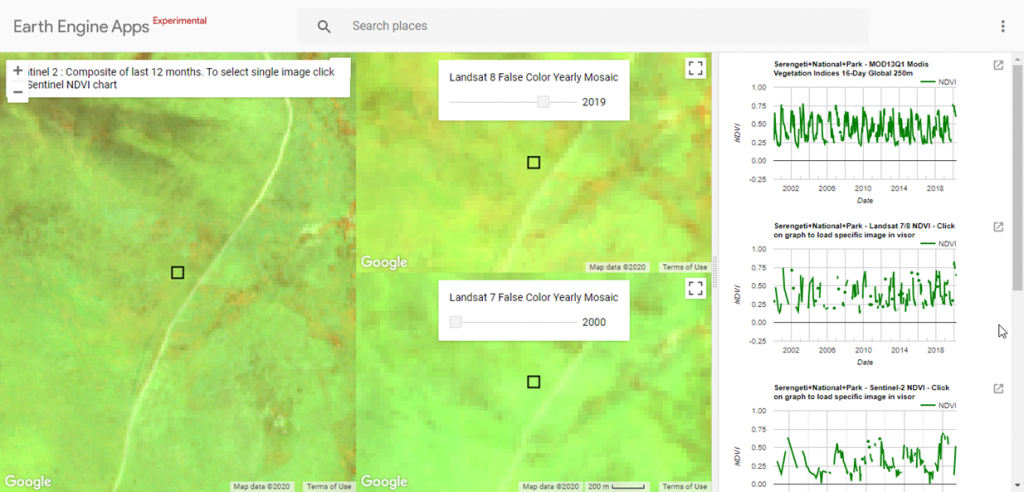
Which satellite images and graphics can you find in the GEE app?
Images: Sentinel 2 and Landsat 7/8 False Color Mosaics (NIR-SWIR-Red)
NDVI graphs: MODIS, Landsat 7/8 and Sentinel-2 NDVI (vegetation index showing the vegetation intensity)
Spatial and temporal resolution of satellite images:
| Satellite | Spatial resolution | Temporal resolution | Imagery available since |
| MODIS | Low (250 m) | High (daily revisit time, graph shows less-cloudy image during16 days) | 2000 |
| Landsat 7/8 | High (30m) | Low (16 days revisit time) | 2000 |
| Sentinel 2 | High (20m) | High (5 days revisit time) | 2015 |
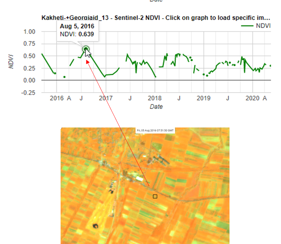
The graphs and the images are connected. Clicking on a certain date in the graph the image of the same day will appear.
But they are not showing the same information!!
The graphs display NDVI values and the false color mosaics show the vegetation intensity.
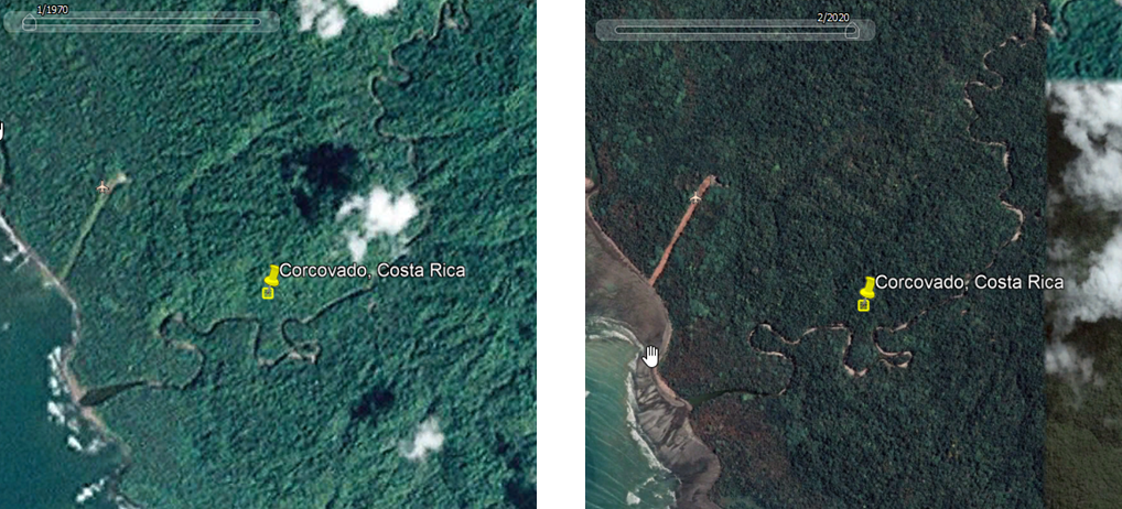
Training plots
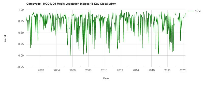
Forest – Broadleaf evergreen (Corcovado, Costa Rica)
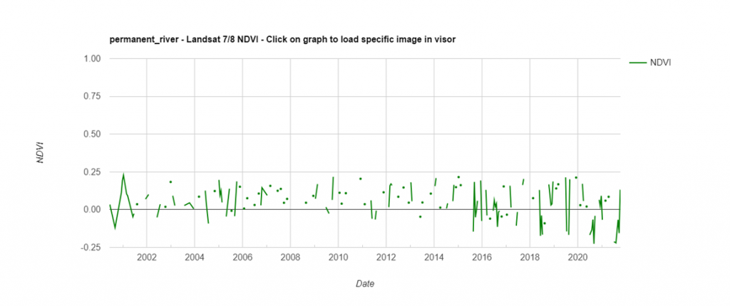
Land use change: Since1970 no changes perceived in terms of forest area and density. The steep drops in the graph are a consequence of the clouds that cover the forest and satellites do not receive the reflection.
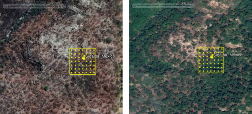
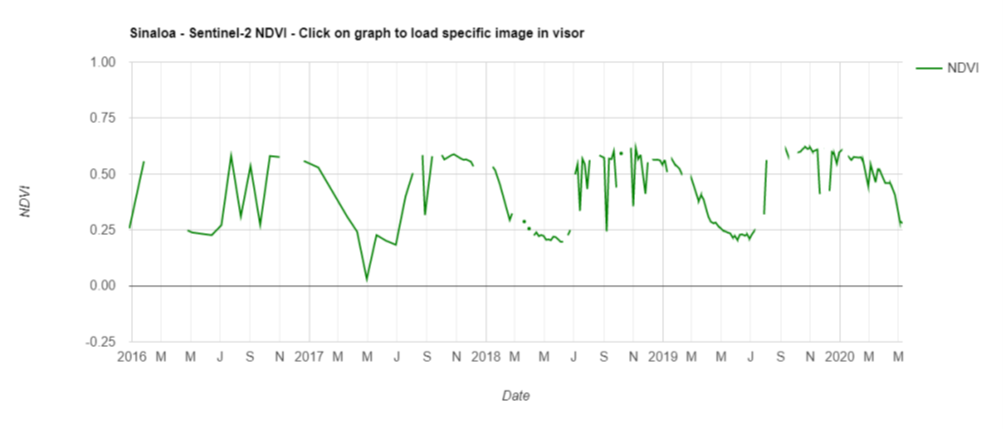
Forest – Broadleaf deciduous (Sinaloa, Mexico)
The NDVI graph shows that the highest NDVI value is above 0,5 and drops till 0,25 in the dry season. Between June and November 2019 the landscape and colors look different due to the fall of the leaves in the deciduous forest.
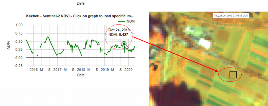
Cropland – Orchard, Vineyard (Kakheti, Georgia)
Looking at the graphic, we will see that vineyards have a particular growing pattern with its highest peak in the summer months and drops after the grapes harvest.
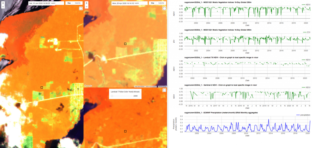
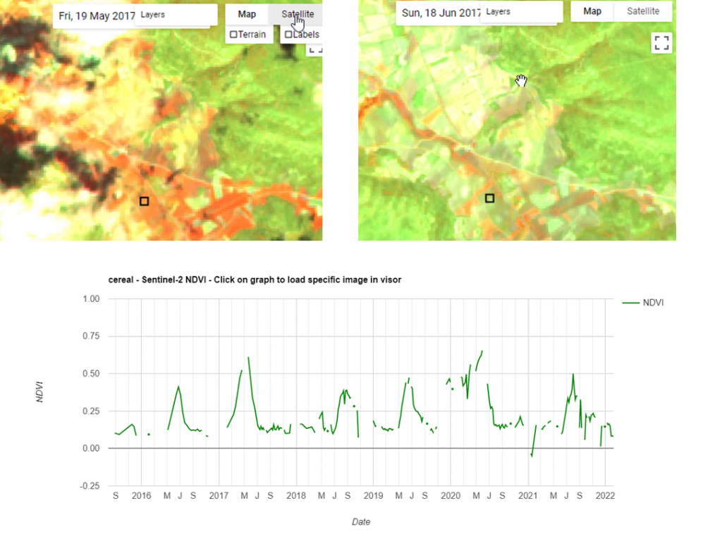
Cropland – Permanent crop, Cereal (Guadalajara, Spain)
Interpretation of Sentinel 2 composite images (20 m resolution) showing the vegetation intensity (orange is high vegetation intensity and green is low vegetation intensity): The image in May 2017 shows its vegetation in its maximal intensity. In the image on the right in June 2017 the vegetation intensity is very low after the harvest.
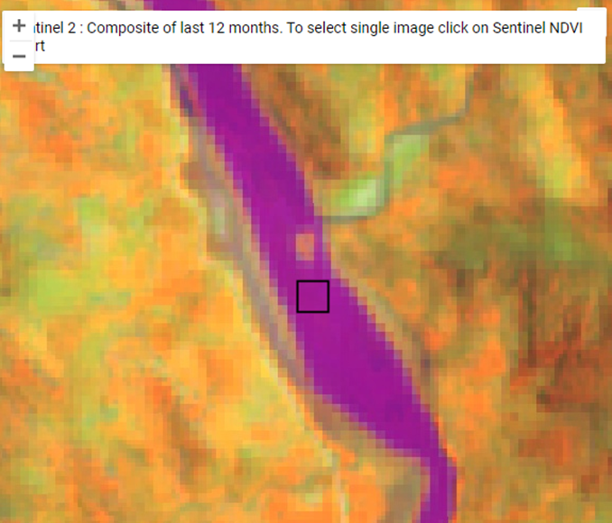
Wetland – Permanent river (Northern- Rwanda, Rwanda)
In this Sentinel image water is represented in purple. The color of the water is purple and not black/dark blue due to the fact that it is a river with shallow waters.
The river is surrounded by areas with healthy vegetation that are represented in orange (orange is high vegetation intensity and green is low